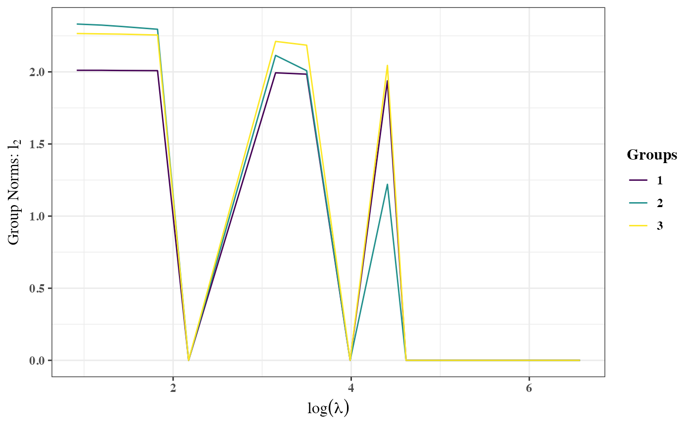
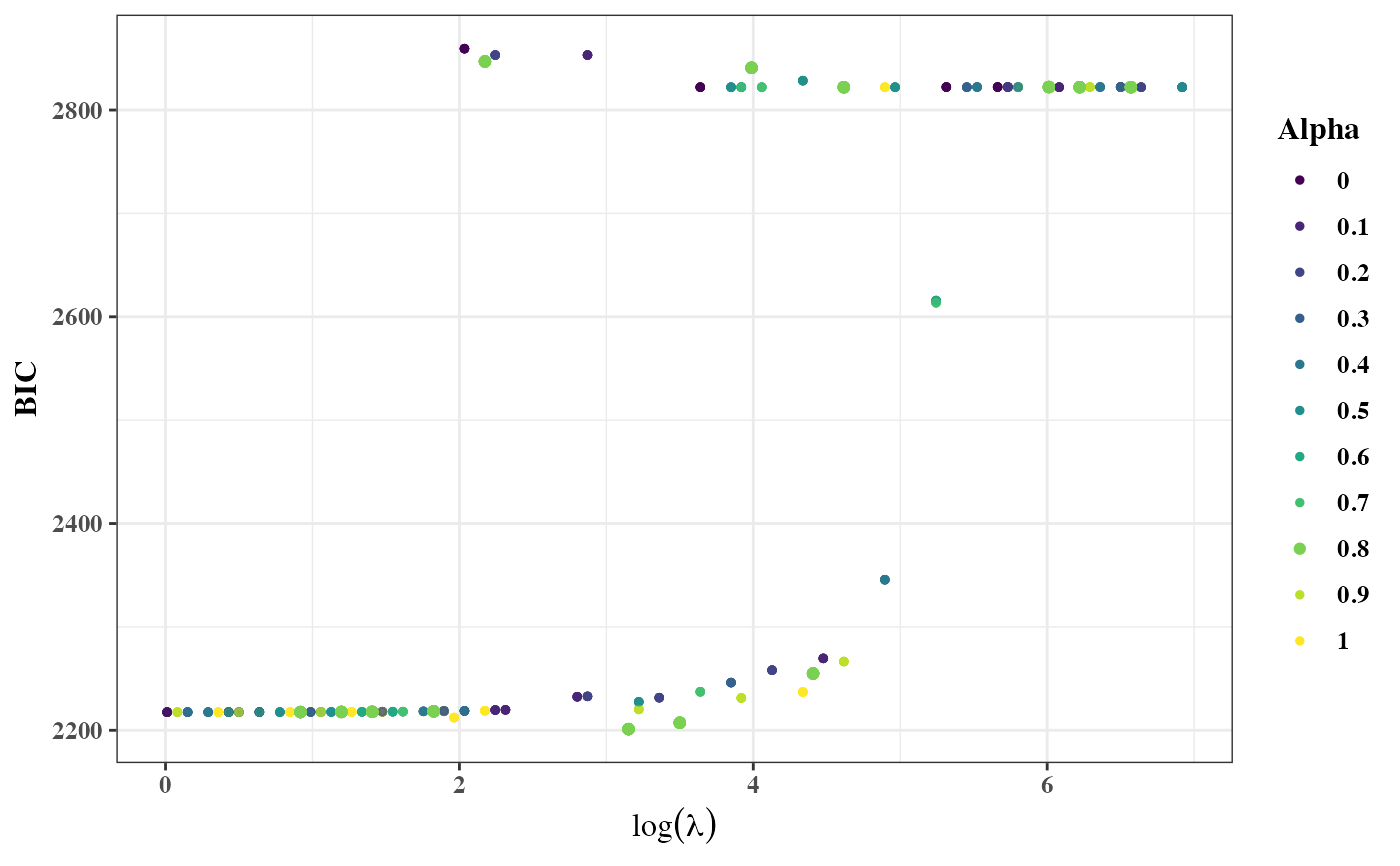
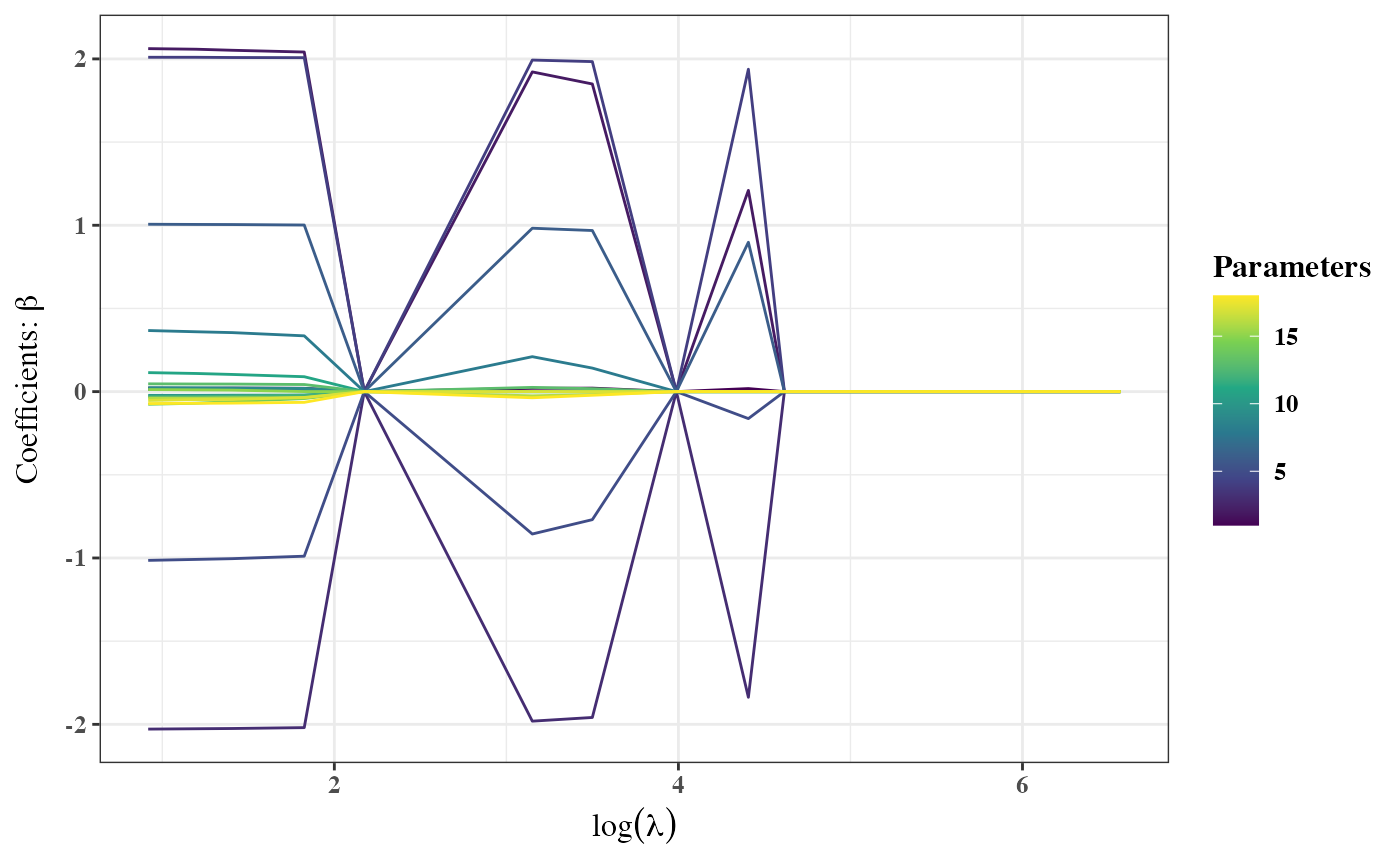
This function creates plots for finite mixture regression models of class FMRM. It generates three plots: lambdas vs. ics for all alpha values, lambdas vs. regression coefficients, and lambdas vs. group norms for all models with the same alpha as the optimal alpha.
Usage
# S3 method for class 'FMRM'
plot(x, ...)Value
A list of three ggplot objects: lambdas vs. ics for all alpha values, lambdas vs. regression coefficients, and lambdas vs. group norms for all models with the same alpha as the optimal alpha.
Examples
set.seed(2025)
# ----Simulate data----
n <- 500 # total samples
p <- 6 # number of covariates
G <- 3 # number of mixture components
rho = 0.2 # correlation
# ----True parameters for 3 clusters----
betas <- matrix(c(
1, 2, -1, 0.5, 0, 0, 0, # component 1
5, -2, 1, 0, 0, 0, 0, # component 2
-3, 0, 2, 0, 0, 0, 0 # component 3
), nrow = G, byrow = TRUE)
pis <- c(0.4, 0.4, 0.2)
sigmas <- c(3, 1.5, 1)/2
# ----Generate correlation matrix----
cor_mat <- outer(1:p, 1:p, function(i, j) rho^abs(i - j))
Sigma <- cor_mat
# ----Simulate design matrix X (n × p)----
X <- mvtnorm::rmvnorm(n, mean = rep(0, p), sigma = Sigma)
# ----Generate responsibilities----
z <- rmultinom(n, size = 1, prob = pis)
groups <- apply(z, 2, which.max)
# ----b0 + b1x1 + b2x2 + ... + bkxp----
mu_vec <- rowSums(cbind(1, X) * betas[groups, ])
# ----Simulate response y----
y <- rnorm(n, mean = mu_vec, sd = sigmas[groups])
# ----Fit model----
mod <- FMRM(x = X,
y = y,
G = 3,
family = gaussian(),
parallel = TRUE,
random = TRUE,
verbose = FALSE)
# ----Call plot----
plots <- plot(mod)
# ----Display plots----
plots[[1]] # ----lambdas vs. ics----
 plots[[2]] # ----lambdas vs. regression coefficients----
 plots[[3]] # ----lambdas vs. group norms----